
Coverage-safe geometry simplification
Our safety and alerting products work with geographic zones: a country, a region, a flood-warning area. A zone is a set of polygons, and those polygons decide, cell by cell, who gets alerted. That last part is what makes this a more interesting problem than it looks. This post is the write-up of a hackathon project that started as “these polygons are too big, let’s simplify them” and ended somewhere more subtle: you cannot simplify a coverage geometry the way you simplify a geometry you only want to draw.
This isn’t the first time we’ve tried. Simplifying dense zones has come back
every few years for well over a decade, and every time it proved harder than it
looked. The routine that actually ran in the product leaned on libgeos'
TopologyPreserveSimplify (via our geom_simplify wrapper), steered by a
tolerance ratio — and in 2018, aimed at France’s regions, it produced outright
invalid geometries: holes escaping their shell, tangled nested rings. Re-running
that exact case on today’s libgeos 3.13 — the same 2016 regions, plus 34,955
communes — the invalidity is simply gone; the failure was bound to an old
libgeos, not to the idea. (The other in-house option, a home-grown
Douglas–Peucker, comes out valid too, but its topology-repair pass is quadratic
in the segment count: it cannot finish on a region the size of metropolitan
France — building that geometry alone exhausts memory.) What the survivors still
do is quietly drop cells. So the honest workaround we handed customers was
“re-cut the zone by hand in QGIS” — effective, but not something you want in the
loop. What changed is that in 2025 a rework of
QKV, our key-value store, solved a performance problem there with a tiny
simplify-then-buffer loop — and that same loop, it turned out, can be generalized
to the other code paths that ingest zones.
The problem
Two of our ingestion paths produce geometries that are far too dense:
- Geocoding (Nominatim): asking for a country or a region hands back a KML polygon with tens to hundreds of thousands of points. Metropolitan France comes back as three polygons totalling 70,555 points — the literal “large input geometry” from the ticket.
- WFS (a GIS server): highly detailed MultiPolygons. One flood-warning area on the Cumbrian coast, at the Duddon estuary, is 226 polygons / 5,367 points spread over a ~22 km bounding box.
Dense geometries are expensive on every axis: to transfer, to render, to edit, and — the one that matters here — to evaluate coverage. Deciding “is this phone inside the zone?” over a 70k-point polygon, for every cell, is not free.
So we simplify. The catch is that the geometry doesn’t just get displayed — it selects the cells. Move a boundary vertex the wrong way and you drop cells that used to be inside the zone. In an alerting product, a dropped cell is a person who does not get warned. That is not a rounding error we get to accept.
What “coverage-safe” means
The usual way to score a simplification is the symmetric difference between the original and the result, or simply the change in area. Both are misleading here, because they lump together two errors that are not remotely equal:
- Under-coverage — area of the original that the simplified zone no longer covers. These are the missed cells. Forbidden.
- Over-coverage — area the simplified zone adds outside the original. We alert a few people who were just outside the zone. An accepted cost.
Once you split the error this way, the whole benchmark changes. An algorithm that only ever grows the zone (inflate-only) has zero under-coverage by construction — it can never drop a cell. A raw symmetric-difference or Δarea metric punishes it for the over-coverage it produces on purpose, and rewards a symmetric algorithm that quietly eats cells. Measuring the wrong thing makes the dangerous option look good.
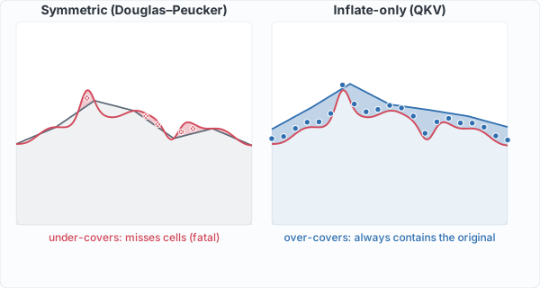
The simplification tolerance is the width of the error band along the boundary. A symmetric algorithm (Douglas–Peucker, left) cuts capes and fills bays alike — the red slivers are original area now outside the stored zone: missed cells. An inflate-only algorithm (right) pushes the boundary strictly outward, so the stored zone always contains the original. It over-covers; it never under-covers.
There is a second way the naive metric lies, and we only hit it on the Cumbrian area: on a fragmented zone, over-coverage also counts the fragments the algorithm merges together — a dissolution we actively want. We come back to that below; keep it in mind, because it flips the reading of one of the tables.
The contenders
We benchmarked the candidates at equal output point count — calibrated by bisection so every algorithm lands on roughly the same number of points. This matters: comparing at equal budget is a trap. At budget 5000 the outer hull overshoots to 5,057 points and then looks about 1.8× more economical on over-coverage, which is not a fair fight. Recalibrated to the same 3,123 points, its real edge is about 23%.
The benchmark runs each algorithm once over the whole placemark (the entire MultiPolygon, exactly as production does), so it exercises the dissolution between neighbouring polygons and lines up with an independent shapely run on the same geometries. Here is France (three polygons, 70,555 points; area 622,745 km²; common target ≈ 3,123 points):
| Algorithm | Time | Pts | Polys | Under | Over |
|---|---|---|---|---|---|
| QKV (inflate-only) | 178 ms | 3,123 | 3→2 | 0 | 0.35% |
| Outer hull (GEOS ≥ 3.11) | 70 ms | 3,123 | 3 | 0 | 0.27% |
| Douglas–Peucker (raw) | 7 ms | 3,123 | 2 | 0.02% | 0.01% |
| Topology-preserving | 71 ms | 3,123 | 3 | 0.02% | 0.01% |
QKV is geom_simplify_to_max_points; the outer hull is
GEOSPolygonHullSimplify (GEOS ≥ 3.11); “topology-preserving” is libgeos
TopologyPreserveSimplify, which the platform’s geom_simplify wraps.
The two symmetric simplifiers are precise and fast, but they miss cells
(under-coverage > 0) — perfectly fine for storage and display, disqualified for
coverage. Only QKV and the outer hull guarantee zero under-coverage, and
of the two, QKV is what we ship on production GEOS 3.8. In absolute terms QKV
over-covers France by 2,180 km² and the hull by 1,681 km² (~23% less); an
independent shapely run cross-checks these — QKV 3,126 points / 2,207.6 km²
(0.354%), the hull ≈ 1,697 km² at equal points. QKV is also the slowest of the
safe options at 178 ms, about 25× a single raw Douglas–Peucker pass: that is the
assumed cost of iterating simplify + buffer + contains until the result
provably wraps the original.
The winner came from the key-value store
The winner wasn’t something we invented for the hackathon. It came out of
QKV, our key-value store — which is where the “QKV” label in the table comes
from. When a geometry is written to QKV, the store keeps, next to the full
geometry, a lightweight simplified copy so that spatial queries don’t have to
chew through hundreds of thousands of points every time. A year before this
hackathon (commit 6af6c2c, July 2025), a colleague had reworked how that copy
is built. The old version was a single symmetric simplify() at a fixed
tolerance, and it had two problems: it didn’t reliably cut the point count, and
it almost never contained the original. The rework turned it into an iterative
simplify-then-buffer loop that stops only once the result both fits a point
budget and contains the original:
- Start small:
simplify(tol)at ~11 m, thenbuffer(2·tol). - If the result is ≤ budget points and contains the original → stop.
- Otherwise multiply the tolerance and buffer by 4 and retry, up to 4 rounds.
- If it never converges, keep the original (fail-safe).
That containment condition is the whole point. For QKV it means the cheap copy
can never exclude a point the real geometry includes, so a query built on it
never returns a false negative. That is exactly the guarantee coverage needs
on the ingestion side — never drop a cell — which is why the benchmark kept
pointing back at an algorithm that already existed in the store. The hackathon’s
real contribution was recognizing the match, lifting the loop out of
qkv/geom.c into a shared geom_simplify_to_max_points in the platform services
geometry module, and wiring it into the paths that ingest zones.
The loop is cumulative — each round simplifies and buffers the previous result, not the original — and it stops as soon as the result is light enough, so the tolerance it settles on is the smallest one that works and the inflation is minimal. On France:
| Round | simplify | buffer | Outcome |
|---|---|---|---|
| 1 | ~11 m | ~22 m | over budget, contains → ×4 |
| 2 | ~44 m | ~88 m | over budget → ×4 |
| 3 | ~178 m | ~356 m | ≤ 5000 ✓, contains ✓ → stop (3,123 pts) |
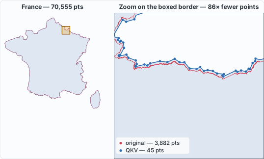
Left: the whole country. Right: a zoom on the boxed stretch of border — the original’s dense vertices (red, 3,882 in this window) against QKV’s 45 (blue), tracing the same line. Overall 70,555 → 3,123 points (−95.6%), zero under-coverage, +0.35% area, three polygons dissolved to two. At country scale the over-coverage is imperceptible; the point reduction is not.
The loop isn’t perfect: at a tight budget on a huge single polygon it can fail to converge within its four rounds and fall back to the original. Its guarantee is “zero under-coverage”, not “always hits the budget” — at budget 5000 on these zones it converges.
Fragmented zones: when over-coverage is the feature
The buffer step has a second, useful effect: it dissolves neighbouring fragments. On the Cumbrian flood-warning area, the 226 tiny polygons merge as the buffer bridges the gaps between them.
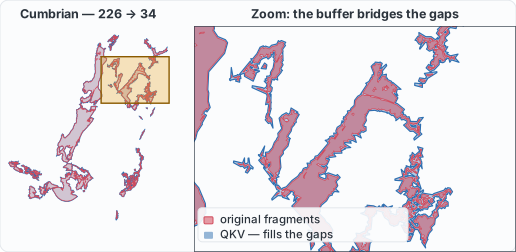
Left: the whole zone, 226 → 34 polygons (target ≈ 4,303 points, +35.6% area). Right: a zoom on one cluster — red fragments with the QKV envelope (blue) filling the channels between them. The symmetric simplifiers can’t do this; each fragment keeps its own minimal ring, so they stay stuck at 226 polygons.
Here is the Cumbrian table, same equal-points calibration:
| Algorithm | Time | Pts | Polys | Under | Over |
|---|---|---|---|---|---|
| QKV | 22 ms | 4,303 | 226→34 | 0 | 35.61% |
| Outer hull | 2.7 ms | 4,303 | 226 | 0 | 2.78% |
| Douglas–Peucker (raw) | 6.8 ms | 4,303 | 210 | 1.16% | 1.05% |
| Topology-preserving | 5.8 ms | 4,303 | 226 | 1.26% | 1.22% |
You would be tempted to read that first-vs-second row as “the hull crushes QKV,
2.78% against 35.61%”. It doesn’t. Most of QKV’s over-coverage is the
dissolution we want: it fuses 226 near-touching fragments into 34 (the
Polys column), which is cleaner and means far fewer objects to index
downstream. The hull scores 2.78% precisely because it refuses to dissolve —
it keeps all 226 polygons, which is operationally worse. So on a fragmented
zone, “over-coverage %” is not a quality score, and QKV is preferred despite
the larger number.
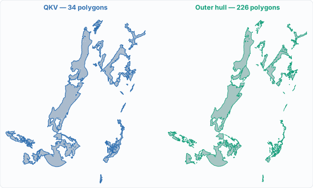
Same point budget, same zero under-coverage. Left: QKV welds the estuary’s 226 fragments into 34 polygons. Right: the outer hull hugs each fragment tightly — its low over-coverage comes entirely from keeping 226 separate pieces, not from being more faithful.
(One honest caveat: not all of the 35.6% is useful dissolution — the ~20 m buffer also thickens the thinnest slivers. Separating “gaps filled” from “edges thickened” would be a refinement of the benchmark.)
That merging is a double-edged sword on small, fragmented zones. Tighten the budget to 2000 and the Cumbrian area collapses to 9 polygons / 872 points — over-coverage climbs as the buffer has to swallow more of the water between the fragments to weld them together. On a big single polygon like France that never happens, which is also why the outer hull’s low-over-coverage advantage only materializes on continuous zones: there is nothing to dissolve, so its minimal envelope is a genuine ~23% win.
What shipped
The simplification runs server-side, on the way in. Most sources (geocoding, WFS, the wizard, manual drawing) converge on a single persistence RPC, so wiring the pass there covers all of them at once; the interactive KML import had its own path, which we covered by factoring the simplification into a shared helper rather than duplicating it. Result geometries that report coverage stay symmetric — inflating a result would be reporting coverage you don’t have. The rule is: an input that selects cells gets inflate-only; a result that reports gets symmetric.
The shipped engine is geom_simplify_to_max_points (the QKV loop above), driven
by a point budget rather than a tolerance ratio. That distinction is the
crux. The older geom_simplify took a ratio — a percentage of the geometry’s
bounding-box diagonal, turned into a tolerance in degrees and clipped between
~10 m and ~500 m — and picking that percentage was guesswork: too small and a
huge zone stays huge, too large and a small one collapses. A point budget instead
targets the actual cost (≤ N points) and self-tunes — the found tolerance is the
smallest that works — whatever the zone’s size. The budget is exposed as a single
simplifyMaxPoints field (0 = off) on every entry point, and the feature is
off by default everywhere: turning it on is a product decision, not something
we flip silently under existing zones.
On today’s production GEOS 3.8, QKV is the right answer. The benchmark also turned up two native GEOS primitives that aim squarely at this problem, both out of reach until we upgrade:
GEOSPolygonHullSimplify(GEOS ≥ 3.11) — a topological outer hull: contains the original by construction, budgeted as a vertex fraction, and adds no new points. On a continuous zone it over-covers ~23% less than our buffered QKV at equal points (1,681 vs 2,180 km² on France). It does not dissolve fragments, though, so it is the wrong tool on a shattered input like Cumbrian, where the dissolution is exactly what we want.GEOSCoverageSimplifyVW(GEOS ≥ 3.12) — simplifies a tiling (adjacent administrative units) without opening gaps or overlaps at shared borders, something we have nothing equivalent for. It is symmetric, though, so it is a storage/display tool, not a coverage-safe one.
Both need a GEOS upgrade (3.8 → 3.1x) that we have not done — doing it properly means reviewing the whole 3.8-to-current diff for behavioural and API changes, which is a project in its own right. So the outer hull is the target for continuous zones; QKV is what runs in production, and it is the only one of the two that handles fragmented zones.
Takeaway
Coverage flips the usual scoring. What matters isn’t how similar the simplified area is, but whether we dropped a cell — and dropping one is the only outcome we can’t accept, while adding a little area is fine. Our first scoreboard ranked by area similarity and so rewarded exactly the algorithms that quietly eat cells. Splitting the error into under- and over-coverage put the ranking straight, and the answer turned out to be a simplify-then-buffer loop we already had in QKV.
The subtlety we didn’t expect: over-coverage isn’t always pure cost. On the fragmented Cumbrian zone most of it is the fragment-dissolving we actually wanted — so an “over-coverage %” means nothing until you know whether the zone is solid or shattered.
And there’s a quieter lesson. Dense zones had been a manual chore for over a decade — re-cut by hand in an external editor. The loop that finally fit wasn’t a grand redesign: it grew inside the key-value store barely a year earlier, for its own performance reasons, and only needed to be recognized, lifted into a shared helper, and wired into the paths that ingest zones. Generalized that way, one loop can serve them all — geocoded countries, WFS flood areas, the alert wizard, interactive KML import — even if switching it on anywhere stays a per-path product decision. On production GEOS 3.8 that loop is what ships; once we upgrade, the outer hull is worth a look on continuous zones.